Impact Factor ISSN: 1449-2288

 Global reach, higher impact
Int J Biol Sci 2012; 8(8):1121-1129. doi:10.7150/ijbs.4866 This issue Cite
Mini-Review
Why Would Plant Species Become Extinct Locally If Growing Conditions Improve?
Koen Kramer1 ![]() , Rienk-Jan Bijlsma1, Thomas Hickler2, Wilfried Thuiller3
, Rienk-Jan Bijlsma1, Thomas Hickler2, Wilfried Thuiller3
1. Alterra, Wageningen University and Research Centre, PO Box 47, 6700 AA Wageningen, Netherlands;
2. Biodiversity and Climate Research Centre, Department of Physical Geography, Goethe-University Frankfurt, Frankfurt am Main, Germany;
3. Laboratoire d'Ecologie Alpine, UMR-CNRS 5553 Université J. Fourier BP 53, 38041 Grenoble Cedex 9, France.
Received 2012-7-12; Accepted 2012-8-28; Published 2012-9-7
Abstract
Two assumptions underlie current models of the geographical ranges of perennial plant species: 1. current ranges are in equilibrium with the prevailing climate, and 2. changes are attributable to changes in macroclimatic factors, including tolerance of winter cold, the duration of the growing season, and water stress during the growing season, rather than to biotic interactions. These assumptions allow model parameters to be estimated from current species ranges. Deterioration of growing conditions due to climate change, e.g. more severe drought, will cause local extinction. However, for many plant species, the predicted climate change of higher minimum temperatures and longer growing seasons means, improved growing conditions. Biogeographical models may under some circumstances predict that a species will become locally extinct, despite improved growing conditions, because they are based on an assumption of equilibrium and this forces the species range to match the species-specific macroclimatic thresholds. We argue that such model predictions should be rejected unless there is evidence either that competition influences the position of the range margins or that a certain physiological mechanism associated with the apparent improvement in growing conditions negatively affects the species performance. We illustrate how a process-based vegetation model can be used to ascertain whether such a physiological cause exists. To avoid potential modelling errors of this type, we propose a method that constrains the scenario predictions of the envelope models by changing the geographical distribution of the dominant plant functional type. Consistent modelling results are very important for evaluating how changes in species areas affect local functional trait diversity and hence ecosystem functioning and resilience, and for inferring the implications for conservation management in the face of climate change.
Keywords: plant species, climate, biogeographical models
Introduction
Models of the geographical range of plant species predict that climate change will have profound impacts (e.g. [1, 2]). The best-known and most used models to evaluate the influence of climate change on species range fall into two classes: statistical climate envelope models and process-based dynamic vegetation models. Both classes assume, firstly, that the range margins of species are determined by macroclimatic factors and, secondly, that the current species range is in equilibrium with the current climate. The model parameters can then be fitted based on the current species range. The explanatory variables used in envelope models include a large array of climatic variables that are assumed to be important, and possible statistical interactions among these variables. The dynamic models commonly include physiological limiting variables that assess cold tolerance, the duration of the growing season and drought tolerance, and competition between species for light, nutrients, water and space. Based on this set of explanatory variables, both approaches can result in a very good match between predicted and observed ranges, thus supporting the two basic assumptions of the species range modelling indicated above. This gives confidence to predict the potential future area of a species, based on climate change scenarios provided by global circulation models. “Potential” then refers in most dynamic models to the condition without dispersal limitation, whereas envelope models usually present the results of both unlimited dispersal and of complete dispersal limitation. In some cases, however, species-specific dispersal is estimated [3].
However, many dynamic forest succession models assume that the maximum growth rate is attained at the core of the geographic distribution of a species and decreases toward its limits [4]. This is the consequence of using a parabolic relationship between growth rate and thermal time (accumulation of days exceeding a temperature threshold, also referred to as Growing Degree Days, GDD) estimated at these limits. In addition, the model assumes that mortality increases with decreasing growth [4]. Thus, in a warmer climate, the growth rate may locally decline concomitantly with increasing temperature sum. Consequently, the model predicts local extinction, even though the growing conditions may actually improve due to the extended growing season.
In this paper we begin by reviewing two major classifications of biogeographical models: envelope models and dynamic models. We show that both the envelope and some dynamic approaches of species area modelling may predict that in the northern hemisphere the southern limit of the species range moves north and the species goes locally extinct on its former southern border even though the growing conditions apparently improve. Secondly, we outline a methodology for modelling biogeographical distributions of perennial plants that would in the future avoid the potential modelling error that we have drawn attention to.
Biogeographical models
Envelope models
Bioclimatic envelope models assume that climate exerts dominant control over the natural distribution of species [5, 6] and that the current species range is in equilibrium with its climatic potential area. If valid, time independent, statistical correlations between climate variables at the limits of the species' geographical distribution can be used to describe current ranges. The potential future range of a species can subsequently be assessed by using future projections of climate change obtained from global circulation models (see [7] for a review).
The approach is based on the concept of the fundamental niche [8] which is defined by the abiotic conditions where the species can survive, grow and reproduce (see [9] for an extensive discussion). Hence, biotic interactions such as competition or predation are not directly considered. Moreover, if only climatic variables are used, what is described is the “climatic niche” rather than the fundamental niche, as the latter is also determined by local abiotic pedological features, such as the pH. The climate envelope is, however, based on observed ranges obtained from presence/absence or abundance data: it is based on the realised niche of a species and does not explicitly consider the conditions the species requires for survival, growth and reproduction. Biotic interactions are thus implicit in the correlation between the species area and the climate [6].
Various advanced statistical techniques are deployed to correlate climate variables with species ranges [10-12]. Additionally, techniques have been developed to refine the climatic envelope to allow more detailed environmental description of fragmented habitat of a species. For example by including generic soil and topographical features [13].Two important advantages of these techniques are that only the current geographical distribution of the species is required (presence/absence data per grid cell) and that the only climate variables required are long-term meteorological averages or variability, and the changes to these predicted by global circulation models. As both data sources are currently widely available, the analysis can be applied to a large number of species and over large areas.
However, some shortcomings of the bioclimatic envelope approach have been pointed out. Davis and co-workers [14, 15] argue that the method is essentially invalid as it fails to consider biotic interactions. These interactions might be essentially true at local scales if neutral assemblages are not the rule [16]. Moreover, if a species has a limited dispersal capacity, its current range might not be in equilibrium with its potential range as determined by climate [17]. A final drawback of correlative envelope models is that they do not include physiological information and hence do not assess differential responses of species to an increased concentration of atmospheric CO2 [14].
Pearson and Dawson [5] refute these objections. Firstly, they point out that bioclimatic envelope models can be highly successful in predicting current species ranges. Secondly, they indicate that for species dispersal it is the rare long-term dispersal events that critically determine the rate of change of geographical areas [18]. These rare events can be assumed to continue and may be becoming less unusual, as humans act as powerful dispersal vectors. Thirdly, Pearson and Dawson argue that envelope models should be seen within a hierarchy of increasingly detailed models when assessing the presence of a species at the scale of the continent, region, landscape or plot. Fourthly, they find that the response of species to elevated CO2 is too complex and uncertain to be included in the models and therefore should be ignored for the time being [5, 19]. But see Rickebusch et al. [20] and Hickler et al. [21] for a recent attempt to account for hydrological effects of increasing atmospheric CO2.
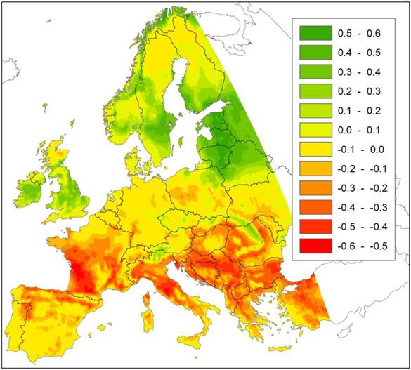
The potential prediction error of local extinction with improving growing conditions that we signal here, in addition to those described above, does not seem to have received attention in the literature. Nevertheless it may have large consequences in some circumstances and for some species. Figure 1 presents an example of a future projection of climate change impact (A2-scenario, [22]) on a species area of European beech (Fagus sylvatica L.) using an ensemble approach of statistical envelope models implemented in the BIOMOD R-package [12, 23] for details). The model predicts a northward shift of the southern limit of beech distribution. For this ensemble of models, the most important factor that cause beech to go extinct locally is growing degree days in August (Figure 2).
Difference in probability of occurrence of European beech under the A2 climate change scenario with that of the current climate, based on an ensemble projection of statistical envelope models (BIOMOD). The map thus represents the change in habitat suitability due to climate change for European beech. Green indicates an increase, red a decrease in habitat suitability relative to the current climate.
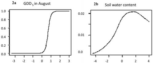
Change in risk of extinction of European beech cause by change in: a. growing degree days (GDD5), or b. soil water content, as function of temperature anomalies (X-axes: difference in temperature between A2 scenario and current climate, ºC). The risk of local extinction strongly increases due to the increase in growing degree days in August, whereas soil moisture has little explanatory power (note different scales of the Y-axes). The predicted reduction of habitat suitability (red areas in Figure 1) is thus mainly caused by the effect of climate change on GDD5.
Dynamic models
Dynamic biogeographical models use bioclimatic variables to constrain the environmental space based on adaptive traits related to a species' ability to survive, and the capacity to gain resources for growth and reproduction, i.e. survival and capacity adaptation [24].
Survival adaptation refers to the physiological traits that improve the likelihood of a species surviving potentially fatal conditions; examples are frost hardiness, drought tolerance, resistance to fire, tolerance to grazing and dormancy of seeds. Dynamic range models usually focus on: i. tolerance of winter cold, ii. winter cold requirements expressed as chilling requirements during the dormant period (together these determine the start of the growing season), and iii. drought tolerance. These three physiological limiting processes related to the survival of plants are discussed in more detail below.
i. Tolerance of winter cold is described by isotherms of the minimum temperature, or the mean temperature of the coldest month [25]. Winter tolerance represents a potential mortality factor, hence a climate change entailing warmer winters means that new habitat will become available and a potential northward shift of the northern limits of a species range can reliably be predicted.
ii. The winter cold requirement (number of chilling days, with mean temperature below 5oC) for bud burst, is often assumed to reduce the thermal time at an exponential rate [26]. As this so-called alternating model [28] is not constrained by a minimum thermal time, it may predict bud burst in the absence of forcing temperature [27]. Additionally, the alternating model is very sensitive to a small variation in the parameter in the exponent, which is difficult to estimate accurately [28], and overestimates the advance of bud burst with increasing temperature [29].
iii. Drought tolerance is often expressed as the ratio of actual evapotranspiration to potential evapotranspiration, which represents moisture availability [30]. Alternatively, in some models drought tolerance is expressed as the relative water content in the soil between wilting point and field capacity during the growing season [31]. Drought stress is a mortality factor that determines the southern and eastern margins of the range of European plant species [32-34].
Capacity adaptation refers to traits that promote resource gain, such as harvesting of light, uptake of nutrients and water, and occupancy of space, all of which improve a species' ability to compete for limiting resources. Dynamic models include extensive process-based descriptions of the uptake and release of carbon, water and nutrients in relation to morphological traits such as growth form and leaf habit, and to physiological traits such as shade tolerance, photosynthetic pathway (C3 or C4) and allocation pattern. Dynamic models usually take a mass-balance approach to resources in the ecosystem. Consequently, actual plant growth is the result of the most limiting resource, given the constraints of the plant's morphological and physiological traits.
Dynamic models that are based on the above described principle of physiologically limiting factors (related to survival and the capacity to gain resources), constrained by morphological features, fall in two broad categories: dynamic vegetation models and dynamic species models. The detail in which these models describe physiological limiting factors, morphological features, population dynamics and competition varies greatly, however, depending on the purpose for which the model has been developed. These models focus on the distribution of plant functional types or biomes at the global scale that are characterised by their physiognomy, such as evergreen vs. deciduous; needle-leaved vs. broad-leaved and different life forms (grass; shrubs; trees) [34-38]. For this paper, however, we focus on the models of perennial plant species.
Dynamic species models almost exclusively address woody species and are referred to as forest succession models [4, 39-41]. They include much mechanistic detail and are therefore more often used to assess a species' response to climate change at a particular location [42] rather than to evaluate climate change impacts on species ranges. Forest succession models are usually based on gap phase replacement of trees, and therefore explicitly take into account conditions for regeneration, competition for light, water and nutrients, and mortality [43]. They may also take into account responses (e.g. growth, seed production and phenology) to elevated CO2 and temperature [33, 44]. Moreover, they allow the impacts of disturbances and changes in disturbance regimes to be explicitly modelled and analysed [45-47]. In the latest generation of forest succession models, sometimes referred to as process-based forest models, growth is modelled as the outcome of physiological processes such as photosynthesis, respiration, leaf and fine root turnover, and allocation of carbon gains to different tissues (e.g. fine roots, sapwood, and leaves) [33, 39, 47]. The different processes are parameterised on the basis of independent measurements, rather than fitted to species ranges. Models of this type preclude the unrealistic prediction that a species will go extinct locally as growing conditions improve. However, they require many parameters that are not easily obtainable from the literature or fieldwork. They do not usually take account of the process of spatial seed dispersal; if they do, they demand much processor time [46].
The dynamic approach based on physiological limiting factors as applied in the process-based forest models has the advantage that responses to climate change have a mechanistic basis and therefore future projections can be assumed to be more reliable than the statistical correlative approach. Also, transient responses of the species to climate change can be reliably simulated. In addition, these models provide the basis for the analysis of ecosystem functioning in terms of cycling of carbon, water and nutrients and the importance of trait diversity for the maintenance and resilience of these functions in the face of climate and land use change [48-52].
However, the species-specific parameters defining the bioclimatic limits are usually not independently determined empirically or by observation, but instead are fitted to the observed species range [53]. This procedure assumes equilibrium between current species occurrences and climate factors, as in envelope models. A classic example is that of relating optimal growth to thermal time (expressed as GDD5) based on a parabolic curve [54] with minimum and maximum GDD5 values fitted to the northern and southern limits of the species area, respectively. The potential risk of this approach is that with increasing growing degree days, the growth rate may decline and attain zero value, thereby producing a predicted northward shift of the southern limit of the species. This can have dramatic consequences for future projections of climate change on a species area depending on the critical upper GDD5 value and the current species distribution (Figure 3). Yet despite this, the approach is still often used to scale up forest succession models developed for the stand scale, to species area [4].
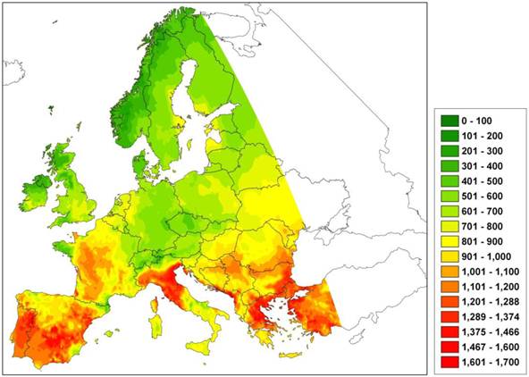
Difference in the number of growing degree days (GDD5) under the A2 climate change scenario with that of the current climate. An increase of GDD5 indicates an increase of the duration of the growing season, thus possibly improved growing conditions. A model using a species-specific GDD5 threshold value to predict a species' geographical area may predict a northward shift of the southern limit with increasing GDD5. Green indicates an increase, red a decrease in GDD5 relative to the current climate.
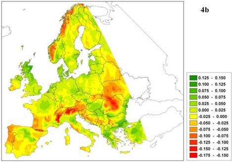
The predicted northward shift of a southern limit is realistic only if the relative competitive ability of the given species decreases with improved environmental conditions, which implies that the southern limit of plant species adapted to warmer climates is determined by biotic interactions [55]. The latest generation of process-based models does determine whether a change in species boundary is caused by physiological constraints (i.e. caused by traits related to survival adaptation) and/or is due to competition (i.e. caused by traits related to capacity adaptation). As an example of such a model outcome, Figure 4 presents the future projection of climate change impact (A2-scenario, [22]) on a species area of European beech (Fagus sylvatica L.) using the dynamic species model LPJ-GUESS [33, 47]. The model predicts a reduction of leaf area index (LAI, Figure 4a) not only in the south and south-east of Europe, but also in the north-west. In this case, the decrease is not caused by higher temperature but by decreasing soil water (Figure 4b) and milder winters, which delays budburst in western beech populations [26] (results not shown). Changes in soil water have a direct effect because in the model the establishment of European beech is constrained by a threshold for the average growing-season soil water content. Milder winters have an indirect effect through competition with other species, which can take more advantage of the warmer climate because budburst is less delayed by the milder winters. Thus in this example, the capacity adaptation of beech is less than that of its competitors. In other words, the process model confirms the results obtained from the statistical model (see Figure 1), but for entirely different reasons.
a. Difference in leaf area index (LAI, m2 leaf surface per m2 soil surface representing leafiness of the beech forest) of European beech under the A2 climate change scenario with that of the current climate. b. Difference in relative soil moisture content ([0-1]) under A2 climate change scenario and the current climate. Green indicates an increase of LAI or relative soil moisture, respectively, red indicates a decrease relative to the current climate.

Methodology for future modelling of the biogeographical distribution of perennial plants
To avoid predicting local extinction despite improved growing conditions for perennial plants, we propose a method in which the future projections of the envelope models are constrained by changes in the geographical distribution of dominant plant species assessed by a dynamic species model on dominant plant species. The null-model, without biotic interactions, can be tested on a species' current range that provides data for validating the model. A mismatch between the observed and predicted species ranges indicates the importance of biotic interactions with other species: if these turn out to be important, the null model is not a suitable tool for assessing the impacts of climate change on the future range of the species, and species interactions should be taken into account.
The statistical bioclimatic envelope models could be applied to a large number of the plant species within the future projection of dominant species made by the dynamic species models. The importance of biotic explanatory factors can be assessed by examining how much the model's goodness-of-fit improves when supposedly important biotic variables are added to the bioclimatic model [56, 57]. In addition, consistency between statistical and dynamic modelling approaches can be tested if the species is actually physiological constrained by the particular climate envelope.
Though both dynamic models of dominant species and statistical envelope models are well-established, there is little harmonisation in the current attempts to refine their selection of explanatory variables. To avoid the potential modelling error that local species extinction is predicted despite improved growing conditions, data can be exchanged between models in order to assess the importance of biotic interactions and to check for consistency of the models' forecasts [58, 59]. Moreover, it is useful to analyse the models' responses to changes in climatic drivers in terms of changes in morphological and physiological traits and diversity thereof: such an analysis can be based on the current theory on ecosystem functioning based on functional trait diversity (i.e. diversity of response and effect traits) [48-50, 52, 60, 61] instead of on a particular species composition. In that way, predictions of range shift of the geographic distribution of dominant plant species can be downscaled to assess changes in functional trait diversity within ecosystems and their consequences for the functioning and resilience of ecosystems in the face of climate change.
We believe that for policy making that anticipates climate change it is important to model the range shifts of species in a consistent way, as only then will the implications of climate change for the functioning of ecosystems be properly understood. This requires closer collaboration between research communities working with different modelling approaches. Instead of building a model that integrates dynamic species modelling and statistical species modelling it will be necessary for these research communities to co-ordinate the selection of driving variables and to exchange compatible data.
Acknowledgements
The discussions and comments by Eric Arets, Richard Bradshaw, Csaba Matyas, Wim Ozinga and Claire Vos are much appreciated. Toon Helmink prepared the maps. KK and RJB were financially supported by the projects DynTerra (project no. KB-14-002-032) and CSR (project no. KB-14-011-007) of the Knowledge Base of the Dutch Ministry of Economics Agriculture and Innovation. WT and TH were partly funded by the EU-FP6 Integrated Project ECOCHANGE (Challenges in assessing and forecasting biodiversity and ecosystem changes in Europe, No:066866 GOCE). WT was supported by the ANR DIVERSITALP project (No. ANR 07-BDIV-014). Joy Burrough advised on the English.
Competing interests
The authors have declared that no competing interest exists.
References
1. Bakkenes M, Alkemade JRM, Ihle F, Leemans R, Latour JB. Assessing effects of forecasted climate change on the diversity and distribution of European higher plants for 2050. Global Change Biology. 2002;8:390-407
2. Thuiller W, Lavorel S, Araújo MB, Sykes MT, Prentice IC. Climate change threats to plant diversity in Europe. Proceedings of the National Academy of Sciences of the United States of America. 2005;102:8245-50
3. Midgley GF, Hughes GO, Thuiller W, Rebelo AG. Migration rate limitations on climate change induced range shifts in Cape Proteaceae. Diversity and Distributions. 2006;12:555-62
4. Bugmann H. A review of forest gap models. Climatic Change. 2001;51:1573-480
5. Pearson RG, Dawson TP. Predicting the impacts of climate change on the distribution of species: are bioclimate envelope models useful? Global Ecology and Biogeography. 2003;12:361-71
6. Guisan A, Thuiller W. Predicting species distribution: offering more than simple habitat models. Ecology Letters. 2005;8:993-1009
7. Heikkinen RK, Luoto M, Araújo MB, Virkkala R, Thuiller W, Sykes MT. Methods and uncertainties in bioclimatic envelope modeling under climate change. Progress in Physical Geography. 2006:30
8. Hutchinson MF. Concluding remarks. Cold Spring Harbour Symposia on Quantative Biology. 1957:415-27
9. Soberón J. Grinnellian and Eltonian niches and geographic distribution of species. Ecology Letters. 2007;10:1115-23
10. Elith J, Graham CH, Anderson RP, Dudik M, Ferrier S, Guisan A. et al. Novel methods improve prediction of species' distributions from occurrence data. Ecography. 2006;29:129-51
11. Phillips SJ, Anderson RP, Schapire RE. Maximum entropy modeling of species geographic distributions. Ecological Modelling. 2006;190:231-59
12. Thuiller W, Lafourcade B, Engler R, Araujo MB. BIOMOD - A platform for ensemble forecasting of species distributions. Ecography. 2009;3:369-73
13. Randin CF, Engler R, Normand S, Zappa M, Zimmerman NE, Pearman PB. et al. Climage change and plant distribution: local model predict high-elevation persistence. Global change Biology. 2009;15:1557-69
14. Davis AJ, Jenkinson LS, Lawton JH, Shorrocks B, Wood S. Making mistakes when predicting shifts in species range in response to global warming. Nature. 1998;391:783-6
15. Davis AJ, Lawton JH, Shorrocks B, Jenkinson LS. Individualistic Species Responses Invalidate Simple Physiological Models of Community Dynamics under Global Environmental Change. Journal of Animal Ecology. 1998;67:600-12
16. Chave J. Neutral theory and community ecology. Ecology Letters. 2004;7:241-53
17. Svenning J-C, Skov F. Limited filling of the potential range in European tree species. Ecology Letters. 2004;7:565-73
18. Higgins SI, Richardson DM. Predicting Plant Migration Rates in a Changing World: The Role of Long-Distance Dispersal. American Naturalist. 1999;153:464-75
19. Thuiller W, Midgley GF, Hughes GO, Bomhard B, Drew G, Rutherford MC. et al. Endemic species and ecosystem vulnerability to climate change in Namibia. Global Change Biology. 2006;12:757-76
20. Rickebusch S, Thuiller W, Hickler T, Araujo MB, Sykes MT, Schweiger O. et al. Incorporating the effects of changes in vegetation functioning and CO2 on water availability in plant habitat models. Biology Letters. 2008 4
21. Hickler T, Fronzek S, Araújo MB, Schweiger O, Thuiller W, Sykes MT. An ecosystem-model-based estimate of changes in water availability differs from water proxies that are commonly used in species distribution models. Global Ecology & Biogeography. 2009;18:304-13
22. Nakicenovic N, Swart R. Emission Scenarios. Cambridge: Cambridge University Press. 2000
23. Marmion M, Parviainen M, Luoto M, Heikkinen RK, Thuiller W. Evaluation of consensus methods in predictive species distribution modelling. Diversity and Distributions. 2009;15:59-69
24. Levitt J. Growth and survival of plants at extremes of temperature - a unified concept. HW Woolhouse (ed): Dormancy and Survival Nr XXIII, Symposia of the society for experimental biology Cambridge University Press p 395-448. 1969
25. Sakai A, Larcher W. Frost survival of plants. Berlin Heidelberg: Springer Verlag. 1987
26. Murray MB, Cannell MGR, Smith RI. Date of budburst of fifteen tree species in Britain following climatic warming. Journal of Applied Ecology. 1989;26:693-700
27. Kramer K. A modelling analysis of the effects of climatic warming on the probability of spring frost damage to tree species in The Netherlands and Germany. Plant, Cell & Environment. 1994;17:367-77
28. Kramer K. Selecting a model to predict the onset of growth of Fagus sylvatica. Journal of Applied Ecology. 1994;31:172-81
29. Kramer K. Phenotypic plasticity of the phenology of seven European tree species in relation to climatic warming. Plant, Cell & Environment. 1995;18:93-104
30. Prentice IC, Sykes MT, Cramer W. A simulation model for the transient effect of climate change on forest landscape. Ecological modelling. 1993;65:51-70
31. Landsberg JJ, Waring RH. A generalised model of forest productivity using simplified concepts of radiation-use efficiency, carbon balance and partitioning. Forest Ecology and Management. 1997;95:209-28
32. Dahl E. The phytogeography of Northern Europe: British Isles, Fennoscandia, and adjacent areas. Cambridge University Press. 1998
33. Smith B, Prentice IC, Sykes MT. Representation of vegetation dynamics in the modelling of terrestrial Ecosystems: comparing two contrasting approaches within European climate space. Global Ecology and Biogeography. 2001;10:621-37
34. Prentice C, Bondeau A, Cramer W, Harrison SP, Hickler T, Lucht W. et al. Dynamic global vegetation modelling: quantifying terrestrial ecosystem responses to large-scale environmental change. In: (ed.) Canadell JG, Pataki D, Pitelka LF. Terrestrial Ecosystems in a Changing World. Berlin: Springer. 2006:175-92
35. Woodward FI. Tansley Review No. 41. Predicting plant responses to global environmental change. New Phytol. 1992;122:239-51
36. Cramer W, Bondeau A, Woodward FI, Prentice IC. et al. Global response of terrestrial ecosystem structure and function to CO² and climate change: results from six dynamic global vegetation models. Global Change Biology. 2001;7:357-73
37. Prentice IC, Monserud RA, Smith TM, Emanuel WR. Modeling Large-Scale Vegetation Dynamics. Vegetation Dynamics & Global Change. 1993:235-50
38. Hickler T, Vohland K, Feehan J, Miller PA, Smith B, Costa L. et al. Projecting the future distribution of European potential natural vegetation zones with a generalized, tree species-based dynamic vegetation model. Global Ecology and Biogeography. 2012;21:50-63
39. Kramer K, Buiteveld J, Forstreuter M, Geburek T, Leonardi S, Menozzi P. et al. Bridging the gap between ecophysiological and genetic knowledge to assess the adaptive potential of European beech. Ecological Modelling. 2008;216:333-53
40. Lischke H, Zimmermann NE, Bolliger J, Rickebusch S, Löffler TJ. Treemig: A forest-landscape model for simulating spatio-temporal patterns from stand to landscape scale. Ecological Modelling. 2006:199
41. Pacala SW, Canham CD, Saponara J, Silander JA Jr, Kobe RK, Ribbens E. Forest models defined by field measurements: Estimation, error analysis and dynamics. Ecological Monographs. 1996;66:1-43
42. Badeck FW, Lischke HK, Bugmann H, Hickler T, Hönninger K, Lasch P. et al. Tree species composition in European pristine forests. Comparison of stand data to model predictions. Climatic Change. 2001;51:307-47
43. Shugart HH, West DC. Forest Succession Models. Bioscience. 1980;30:308-13
44. Van der Meer PJ, Jorritsma ITM, Kramer K. Assessing climate change effects on long term forest development: adjusting growth, phenology, and seed production in a gap model. Forest Ecology and Management. 2002;62:39-52
45. Prentice IC, Sykes MT, Cramer W. The possible dynamic response of northern forests to global warming. Global Ecology and Biogeography Letters. 1991;1:129-35
46. Kramer K, Groen TA, van Wieren SE. The interacting effects of ungulates and fire on forest dynamics: an analysis using the model FORSPACE. Forest Ecology and Management. 2003;181:205-22
47. Hickler T, Smith B, Sykes MT, Davis MB, Sugita S, Walker K. Using a generalized vegetation model to simulate vegetation dynamics in northeastern USA. Ecology. 2004;85:519-30
48. Chapin FS, Rincon E, Huante P. Environmental Responses of Plants and Ecosystems as Predictors of the Impact of Global Change. Journal of Biosciences. 1993;18:515-24
49. Chapin FSI, Walker BH, Hobbs RJ, Hooper DU, Lawton JH, Sala OE. et al. Biotic control over the functioning of ecosystems. Science. 1997;227:500-4
50. Lavorel S, Garnier E. Predicting changes in community composition and ecosystem functioning from plant traits: revisiting the Holy Grail. Functional Ecology. 2002;16:545-56
51. Naeem S. Species redundancy and ecosystem reliability. Conservation Biology. 1996;12:39-45
52. Smith TM, Shugart HH, Woodward FI, Burton PJ. Plant functional types. In: (ed.) Solomon AM, Shugart HH. Vegetation Dynamics & Global Change. New York: Chapman Hall. 1993:272-292
53. Sykes MT, Prentice IC, Cramer W. A bioclimatic model for the potential distributions of north European tree species under present and future climates. Journal of Biogeography. 1996;23:203-33
54. Smith TM. Examining the consequences of classifying species into functional types: as imulation model analysis. In: (ed.) Smith TM, Sugart HH, Woodward FI. Plant Functional Types Their relevance to ecosystem properties and gobal change. Cambridge University Press. 1997:319-41
55. Loehle C. Height growth rate tradeoffs determine northern and southern range limits for trees. Journal of Biogeography. 1998;25:735-42
56. Araujo MB, Luoto M. The importance of biotic interactions for modelling species distributions under climate change. Global Ecology and Biogeography. 2007;16:743-53
57. Hughes GO, Thuiller W, Midgley GF, Collins K. Environmental change hastens the demise of the critically endangered riverine rabbit (Bunolagus monticularis). Biological Conservation. 2008;141:23-34
58. Thuiller W, Albert C, Araujo MB, Berry PM, Cabeza M, Guisan A. et al. Predicting global change impacts on plant species' distributions: Future challenges. Perspectives in Plant Ecology, Evolution and Systematics. 2008;9:137-52
59. Jeltsch F, Moloney KA, Schurr FM, Köchy M, Schwager M. The state of plant population modelling in light of environmental change. Perspect Plant Ecol Evol Syst. 2008;9:171-89
60. Naeem S, Thompson LJ, Jones TH, Lawton JH, Lawler SP, Woodfin RM. Changing community composition and elevated CO2. In: (ed.) Korner C, Bazzaz FA. Carbon Dioxide, Populations, and Communities. Academic Press Inc. 1996:93-100
61. Naeem S, Hakansson K, Lawton JH, Crawley MJ, Thompson LJ. Biodiversity and plant productivity in a model assemblage of plant species. Oikos. 1996;76:259-64
Author contact
![]() Corresponding author: koen.kramernl, +31 317 485873.
Corresponding author: koen.kramernl, +31 317 485873.